CED Sample Exam (p.240–250) + Course Framework Skill 2.B / 4.B 표현 보존 · D-5 정독용
📌 분류:🎨 직접 그리기 = FRQ Skill 2.B "Construct numerical or graphical representations"에서 학생이 그리는 그래프
📖 해석만 = 시험에서 제공됨, Skill 4.B "Interpret"만 평가 (그릴 필요 X)
📌 색상:청록색 = AP Statistics 시그니처
📌 출처: College Board AP Statistics CED V.1 (2020) — Sample Exam Questions p.240–250 + Course Framework Unit 1·2·3·5·6·7·8·9 + Formula Sheet (Appendix p.260–265)
🎨 직접 그리기 — Skill 2.B "Construct numerical or graphical representations"
FRQ에서 "Sketch / Draw / Construct"가 나오면 아래 라벨을 빠짐없이 적어야 한다. 축 라벨 누락은 거의 자동 -1점이다.
1
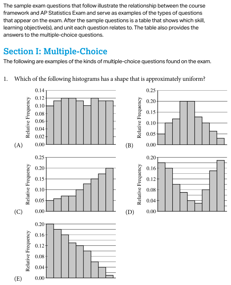
Histogram (히스토그램)
🎨 그리기Unit 1Skill 2.BUNC-1.H
X축 라벨
변수명 (단위) 예: Lead Concentration (ppm), Time (min)
Y축 라벨
Frequency 또는 Relative Frequency (어느 쪽인지 명시)
구간(bin)
등간격 — bin width 일관. 막대 사이 간격 없음 (붙어 있어야 함)
척도(scale)
X축 눈금에 숫자 표시 (예: 0, 50, 100, 150, …)
X축 변수 + 단위, Y축 (Relative) Frequency 라벨
막대 붙어 있음 (bar chart 아님 주의)
분포 모양·중심·퍼짐·이상치(SOCS) 묘사 가능
CED 원문: "In a histogram, the height of each bar shows the frequency or relative frequency of values in the corresponding interval." (CED p.21, Topic 1.4)
📌 자주 틀리는: Y축에 "Frequency"라고만 쓰고 단위 누락 → 감점. relative frequency면 반드시 "Relative Frequency"로 명시.
출처: AP Statistics CED · Sample Exam Q1 · 인쇄 p.240 (file p.247)
2
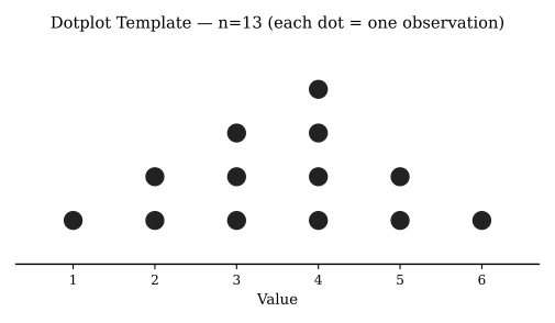
Dotplot (점도표)
🎨 그리기Unit 1Skill 2.BUNC-1.H
X축 라벨
변수명 (단위)
Y축
(없음) — 점이 도수 표현
점
각 관측치 = 점 1개. 같은 값은 위로 쌓는다
척도
X축 눈금 숫자 표시
모든 데이터 점 누락 없이 표시
같은 값은 정확히 수직 정렬해 쌓기
X축 변수명 + 단위
CED 원문: "A dotplot represents each observation by a dot above the corresponding value on a number line." (CED p.21, Topic 1.4)
📌 자주 틀리는: 점을 가로로 흘려서 표시 → 도수 가독성 상실. 반드시 수직 stacking.
출처: Claude SVG (검증 후 제거 가능) — Dotplot 표준 템플릿. 데이터 [1,2,2,3,3,3,4,4,4,4,5,5,6] (n=13). 수직 stacking으로 모드(4) 가독성 확인.
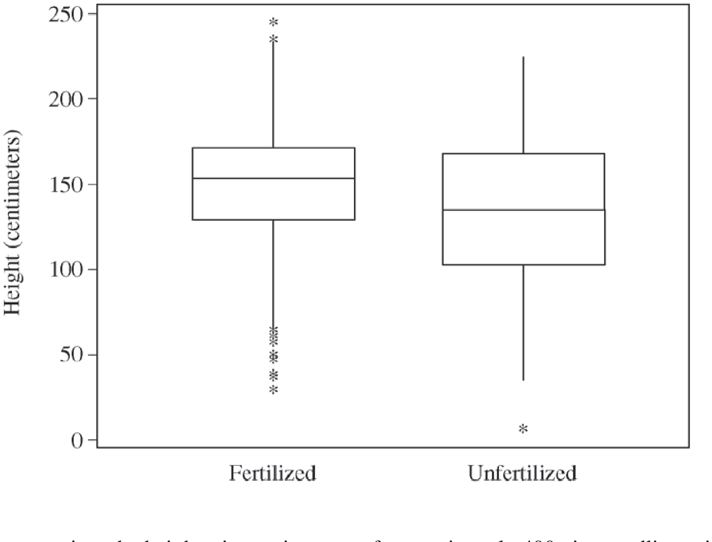
점(•) 또는 별표(*)로 표시 — 점선 X 기준: Q1 − 1.5·IQR 미만 또는 Q3 + 1.5·IQR 초과
whisker
fence 안의 마지막 점까지 직선
5수치 요약 정확 (median 위치 = 50% 지점)
1.5·IQR fence 계산 → 이상치 점으로 분리
축 라벨 + 단위, 척도 표시
CED 원문: "A boxplot is a graphical representation of the five-number summary." (CED p.21, Topic 1.4)
📌 -1점 함정: 이상치를 whisker 끝으로 표시 (점선 연결) → modified boxplot 정의 위반. 반드시 점으로 분리 표시.
출처: AP Stat Mock Test 5 — Seedling 데이터 (Fertilized vs Unfertilized 변형 박스플롯, 이상치 ✱ 표시)
4
Stem-and-Leaf Plot — 줄기-잎 그림
🎨 그리기Unit 1Skill 2.B
줄기(stem)
관측값의 첫 자릿수(들). 세로로 정렬
잎(leaf)
마지막 한 자리. 줄기 옆에 오름차순으로 나열
Key/Legend
필수: 예) Key: 5|3 = 53 minutes
back-to-back
두 그룹 비교 시 좌우 대칭. 왼쪽은 오른쪽이 작은 순(역방향)
Key 표기 (단위 포함)
잎이 정렬되어 있음
back-to-back일 때 왼쪽은 줄기에서 멀어질수록 큰 값
CED 원문: "In a stem and leaf plot, each data value is split into a 'stem' (the first digit or digits) and a 'leaf' (usually the last digit)." (CED p.21, Topic 1.4)
⚠️ Key 표기 누락 = -1점. Stem과 Leaf의 자릿값을 반드시 표시 (예: 5|0 = 50).
5
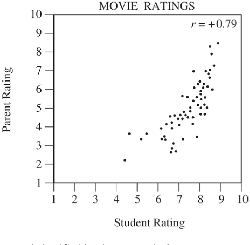
Scatterplot (산점도)
🎨 그리기Unit 2Skill 2.BDAT-1.A
X축
설명변수 (explanatory variable) + 단위
Y축
반응변수 (response variable) + 단위
점
각 (x, y) 쌍 1개
척도
두 축 모두 눈금 + 숫자 표시
X축 = explanatory, Y축 = response 정확히 (혼동 -1점)
축 라벨 + 단위
관계 묘사: form (linear/curved), direction (positive/negative), strength (strong/weak), unusual features
CED 원문: "A scatterplot shows two numeric values for each individual ... can be described as positive, negative, or none." "linear or curved." "form ... direction ... strength" (CED p.46–48, Topic 2.4)
📌 자주 틀리는: 설명변수와 반응변수를 바꿔 그림. "Predict y from x"가 문제 조건이면 x = explanatory.
출처: AP Stat Mock Test 5 — Movie Ratings 산점도 (X=Student Rating, Y=Parent Rating, 양의 강한 선형 r=+0.79)
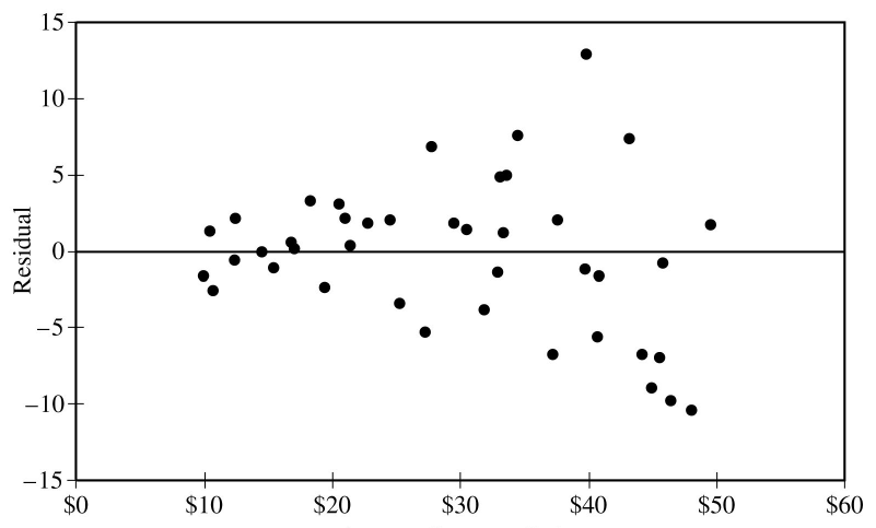
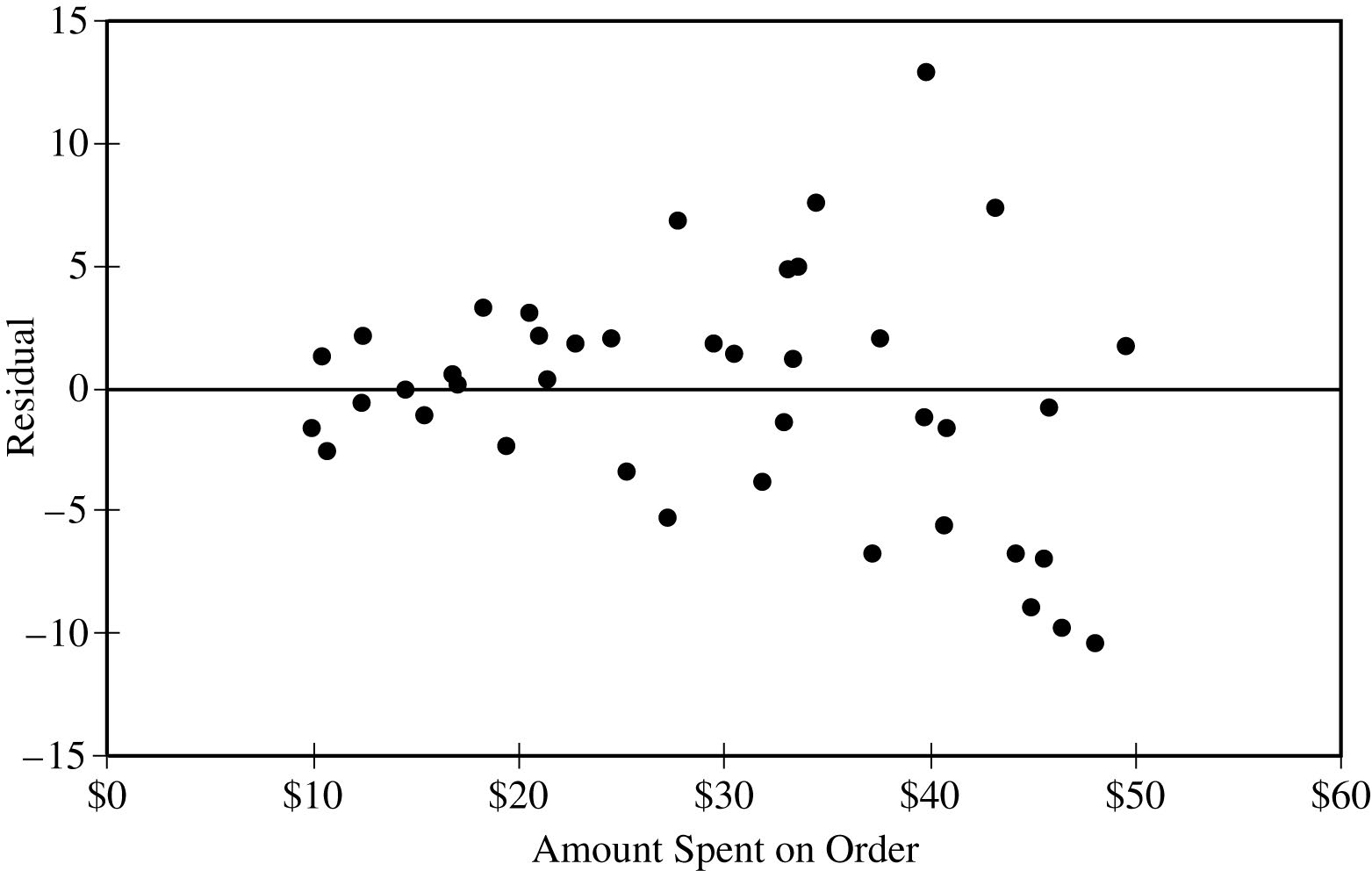
CED 원문: "A residual plot is a plot of residuals versus the explanatory variable or predicted responses." "Apparent randomness in a residual plot ... linear association." (CED p.55, Topic 2.7) "residual = y − ŷ"
📌 자주 틀리는: Y=0 선 누락 → 잔차 부호 판단 어려움. "Residual"이라고 라벨 명시 안 하면 무엇을 그렸는지 채점 불가.
출처: AP Statistics CED · Sample Exam Q15 · 인쇄 p.246 — Y축 "Residual", X축 "Amount Spent on Order ($)"
7
Least-Squares Regression Line (LSRL) with Scatterplot
🎨 그리기Unit 2·9Skill 2.BDAT-1.G
축
X = explanatory, Y = response (단위 포함)
점
관측값 산점도
회귀선
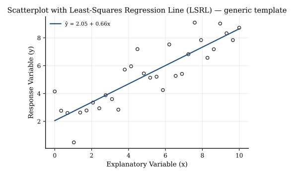
ŷ = a + bx 직선. 식 명시 권장
식 표기
예: ŷ = 65 − 0.70(latitude) (CED Q7 형식)
예측값에 모자(ŷ): "predicted" 표시 필수
변수명을 식에 그대로 (latitude, age 등)
slope 해석: "1단위 변화당 ŷ 평균 b만큼 변화"
CED 원문: "Least-squares regression ... minimizes the sum of the squares of the residuals." (CED p.59, Topic 2.8)
📌 -1점 함정: ŷ를 그냥 y로 표기 (모자 누락). slope 해석에서 "increase"만 쓰고 "average / predicted" 누락 → 인과적 표현 감점.
출처: Claude SVG (검증 후 제거 가능) — LSRL 표준 템플릿 (산점도 + 회귀선 + 식)
8
Normal Distribution Curve — 정규분포 곡선
🎨 그리기Unit 1·5Skill 3.AVAR-2.B
X축 라벨
변수명 (단위) 또는 z (표준화 시)
중심
μ의 위치 표시 + 수치
표준편차 표시
±1σ, ±2σ, ±3σ 위치에 눈금 (68-95-99.7 룰)
음영(shaded area)
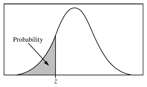
P(X < a), P(X > a) 등 — 색칠 + 확률 라벨
곡선이 좌우 대칭 + 종모양
X축 라벨 + 단위
음영 영역 명확히 채움 (점선 X, 면 채우기 O)
임계값 위치를 X축에 수직선으로 표시
CED 원문: "The area under a normal curve over a given interval is the proportion of values in that interval." (CED p.108, Topic 5.6)
📌 자주 틀리는: X축 라벨 누락 → "어떤 변수의 분포"인지 불명확. z-score만 쓰면 원변수 ↔ z 환산 정보 누락.
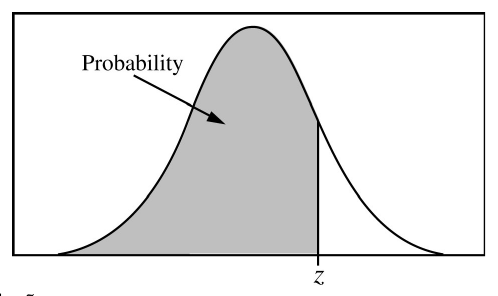
출처: AP Statistics CED · Appendix Table A 머리 그림 · "Probability"·"z" 라벨 표시 방식 (p.262)
9
Sampling Distribution of p̂ — 표본비율의 표본분포
🎨 그리기Unit 5Skill 3.BUNC-3.E
X축 라벨
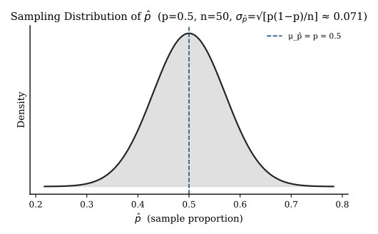
p̂ (Sample Proportion)
중심
μp̂ = p (모비율과 동일)
표준편차
σp̂ = √(p(1−p)/n)
모양
np ≥ 10, n(1−p) ≥ 10이면 근사 정규
X축 = p̂, 곡선 중심 = p
SD 식 정확 (Formula Sheet 참조)
10% 조건 (n ≤ 0.1·N) 명시
Large counts 조건 (np ≥ 10, n(1−p) ≥ 10) 명시
CED 원문: "The sampling distribution of the sample proportion ... is approximately normal when np and n(1−p) are at least 10." (CED Topic 5.5)
📌 자주 틀리는: SE 공식에서 n으로만 나누는 실수 → 반드시 p(1−p)를 곱한 뒤 n으로 나눔. 정규근사 조건(np≥10, n(1−p)≥10) 둘 다 명시 — 한쪽만 쓰면 감점.
출처: Claude SVG (검증 후 제거 가능) — 표본비율 p̂의 표본분포 (p=0.5, n=50, σ_{p̂}=√[p(1−p)/n]≈0.071). 정규근사 조건 만족.
10
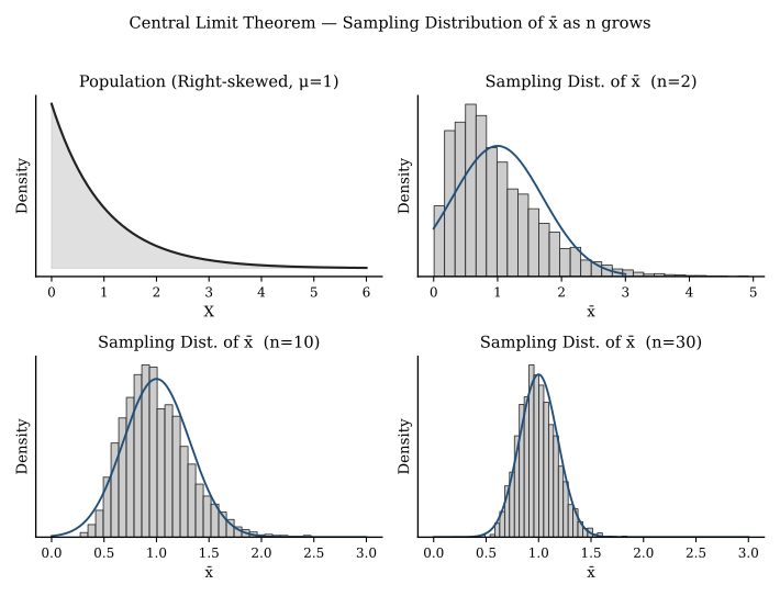
Sampling Distribution of x̄ — 표본평균의 표본분포
🎨 그리기Unit 5Skill 3.BUNC-3.O
X축 라벨
x̄ (Sample Mean)
중심
μx̄ = μ
표준편차
σx̄ = σ/√n
모양
모집단이 정규이거나 n ≥ 30 (CLT)이면 근사 정규
X축 = x̄ (소문자 + bar)
곡선 중심 = μ + 수치
SD = σ/√n (n 누락 X)
CLT 또는 모집단 정규성 근거 명시
CED 원문: "The sampling distribution of a statistic is the distribution of values taken by the statistic in all possible samples of the same size." (CED Topic 5.4)
📌 핵심: n이 커지면 분포가 좁아진다 (SD = σ/√n). 그래프에서 n=10보다 n=100이 더 뾰족해야 함. σ vs σ/√n 혼동(원분포 표준편차로 그리면 X), CLT 조건 n≥30 잊기.
출처: Claude SVG (검증 후 제거 가능) — CLT 핵심: 우편향 모집단 (μ=1)에서 표본평균 분포가 n=2 → 10 → 30로 갈수록 정규에 수렴. 하단 빨간 선은 σ/√n 정규 overlay.
11
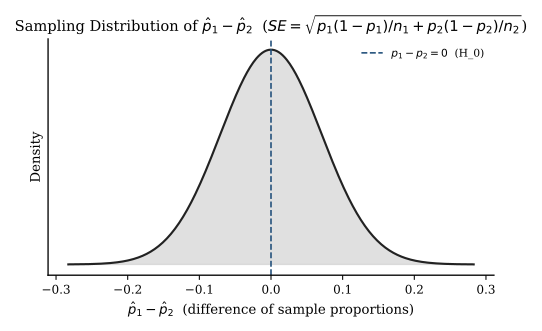
Sampling Distribution of p̂₁ − p̂₂
🎨 그리기Unit 5·6Skill 3.B
X축
p̂₁ − p̂₂
중심
p₁ − p₂
표준편차
σ = √(p₁(1−p₁)/n₁ + p₂(1−p₂)/n₂)
조건
각 표본에 대해 large counts (n₁p₁, n₁(1−p₁), n₂p₂, n₂(1−p₂) ≥ 10)
두 표본의 large counts 조건 모두 검증
독립성 (10% 조건 + 무작위 추출/할당)
SD 식에서 n₁, n₂ 모두 표기
CED 원문: "The sampling distribution for the difference of two independent sample proportions has mean p₁ − p₂ and standard deviation √[p₁(1−p₁)/n₁ + p₂(1−p₂)/n₂]." (CED Topic 5.7 / 6.10)
📌 자주 틀리는: 분산을 합칠 때 차이가 아니라 더하기! SE = √(분산₁ + 분산₂) — 각 표본의 분산을 더한 뒤 √. 또한 양쪽 large counts 조건을 각각 검증해야 함 (한쪽만 만족 → 정규근사 X).
출처: Claude SVG (검증 후 제거 가능) — p₁=p₂=0.5, n₁=n₂=100 가정 시 H₀: p₁−p₂=0 중심 정규분포. SE=√[p(1−p)/n₁ + p(1−p)/n₂].
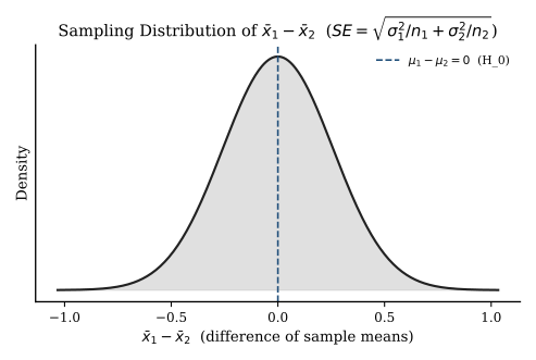
CED 원문: "The sampling distribution for the difference of two independent sample means has mean μ₁ − μ₂ and standard deviation √(σ₁²/n₁ + σ₂²/n₂)." (CED Topic 5.8)
📌 자주 틀리는: SE 공식에서 ÷n 혼동 — σ²/n 형태로 더하고 √. σ²/n₁n₂ 같은 잘못된 형태 X. AP Stat에서는 unpooled SE (Welch's) 사용 권장 — pooled는 두 분산 같다는 강한 가정 필요해 거의 안 씀.
출처: Claude SVG (검증 후 제거 가능) — H₀: μ₁−μ₂=0 중심 표본분포. SE=√(σ₁²/n₁ + σ₂²/n₂). 분산 더하기, 그 후 √.
13
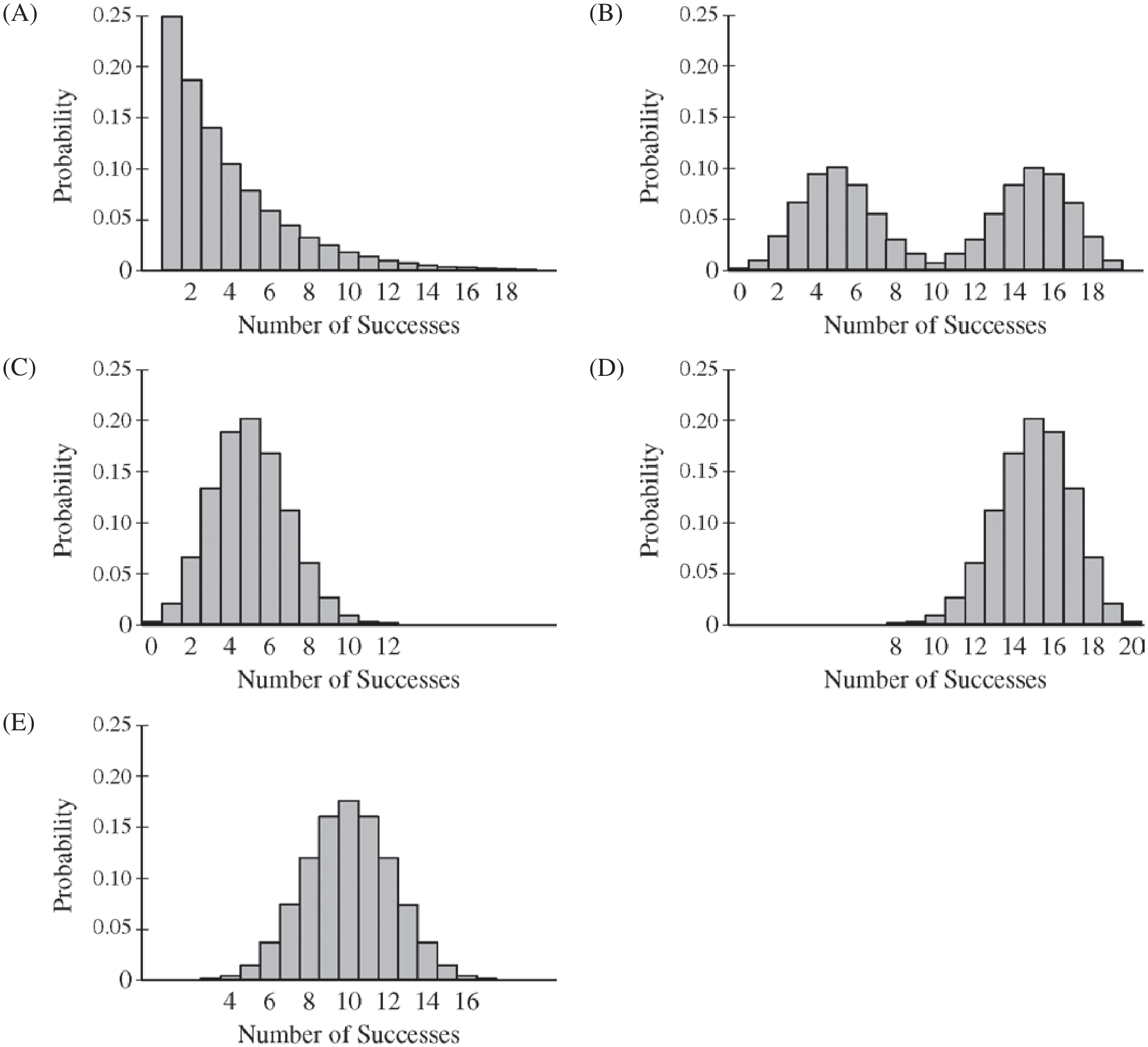
Binomial Distribution PMF — 이항분포 확률질량함수
🎨 그리기Unit 4Skill 3.AUNC-3.B
X축 라벨
x (Number of Successes) — 이산값 0, 1, 2, …, n
Y축 라벨
P(X = x) 또는 Probability
막대
각 x에 대해 P(X=x) 높이의 막대 (붙어 있지 않음 — 이산)
모수
X ~ B(n, p) 명시
X = 0부터 n까지 정수만
p < 0.5면 우편향, p > 0.5면 좌편향, p = 0.5 대칭
μ = np, σ = √(np(1−p))
CED 원문: "If X has a binomial distribution with parameters n and p, then P(X = x) = C(n,x)·px·(1−p)n−x" (Formula Sheet, Appendix p.260)
출처: AP Stat Mock Test 5 Q14 — Binomial PMF 5개 후보 (n=20, p=0.25). 정답은 우편향 + 평균 np=5 근처 봉우리.
14
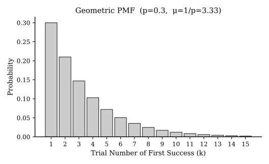
Geometric Distribution PMF — 기하분포 확률질량함수
🎨 그리기Unit 4Skill 3.AUNC-3.B
X축 라벨
x (Trials until first success) — x = 1, 2, 3, …
Y축 라벨
P(X = x)
막대
x가 커질수록 단조 감소 (지수 감소)
모수
X ~ Geom(p)
X 시작 = 1 (0이 아님)
μ = 1/p
식: P(X = x) = (1−p)x−1·p
CED 원문: "If X has a geometric distribution with parameter p, then P(X = x) = (1−p)x−1·p, where x = 1, 2, 3, ..." (Formula Sheet, Appendix p.260)
출처: Claude SVG (검증 후 제거 가능) — Geometric PMF (p=0.3, μ=1/p≈3.33). x=1부터 단조감소.
15
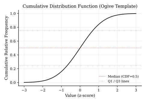
Cumulative Distribution Plot — 누적분포
🎨 그리기Unit 1·5Skill 2.B
X축 라벨
변수명 (단위) 또는 x
Y축 라벨
Cumulative Frequency 또는 Cumulative Relative Frequency (0 ~ 1)
곡선
비감소 step 함수 또는 부드러운 곡선
Y축 끝값이 N(빈도) 또는 1.0(상대빈도)인지 일치
Median(0.5) 위치 → X축 값으로 환산 가능
Q1(0.25), Q3(0.75) 추정 가능
출처: Claude SVG (검증 후 제거 가능) — 누적분포(Ogive). Y=0.5에서 median, Y=0.25/0.75에서 Q1/Q3 환산.
16
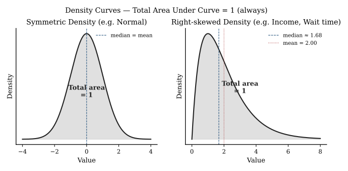
Density Curve — 확률밀도함수
🎨 그리기Unit 1·4Skill 2.BVAR-2.A
X축 라벨
변수명 (단위)
Y축 라벨
Density 또는 f(x)
전체 면적
= 1 (반드시 명시)
음영
P(a < X < b) = a~b 구간 면적
곡선 아래 전체 면적 = 1
곡선이 항상 ≥ 0
특정 구간 확률 = 면적 (음영)
출처: Claude SVG (검증 후 제거 가능) — 두 density 비교: symmetric (정규 같은) vs right-skewed (소득·대기시간 같은). 양쪽 모두 total area = 1. 우편향에서 mean > median.
17
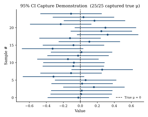
Confidence Interval Visualization — 신뢰구간 다중 표시
🎨 그리기Unit 6·7Skill 4.B
X축 라벨
변수 또는 모수 (예: μ, 추정 단위)
Y축
표본 번호 (sample 1, 2, …, k)
구간
각 표본의 CI를 수평 선분으로 (점 = 표본통계량, 양 끝 = upper/lower bound)
모수선
참 모수 위치에 수직선 (실제 시험엔 모름, 시뮬레이션 그래프용)
"95% Confidence" → 95% 표본의 CI가 모수 포함
해석: "We are 95% confident that the interval (L, U) captures μ"
"95% probability that μ is in the interval"는 틀린 표현
📌 -1점 함정: CI 해석에서 "probability that μ is between L and U" 사용 → 빈도주의 정의 위반. 반드시 "capture / contain the true parameter"로 표현.
출처: Claude SVG (검증 후 제거 가능) — 25개 표본의 95% CI. 약 95% 가 참 모수(점선)를 capture.
18
Power Curve / Type I·II Error 시각화
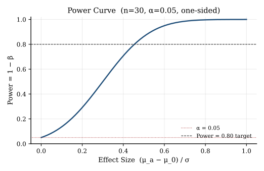
🎨 그리기Unit 6·7Skill 4.EUNC-5.B
두 곡선
H₀ (μ₀ 중심), H₁ (실제 μ 중심) — 각각 정규분포
임계값
α 임계값에서 수직선 — 영역 분리
α (Type I)
H₀ 곡선의 임계값 너머 음영 (귀무 기각 시)
β (Type II)
H₁ 곡선의 임계값 이쪽 음영 (귀무 기각 실패 시)
Power
1 − β = H₁ 곡선에서 임계값 너머 면적
두 분포가 임계값을 사이에 두고 겹침
α 음영(H₀에서) + β 음영(H₁에서) 색 구분
Power 식: 1 − β
n 증가 → β 감소 → Power 증가
CED 원문: "The power of a statistical test is the probability that the test will correctly reject a false null hypothesis." (CED Topic 6.7 / 7.7)
출처: Claude SVG (검증 후 제거 가능) — Power vs effect size (α=0.05, n=30 고정). 0.80 권장선 + α=0.05 baseline.
📖 해석만 — Skill 4.B "Interpret"
시험에서 그래프가 주어지면 해석만 한다. 직접 그릴 필요 없지만 라벨 의미를 빠르게 읽어내야 한다.
1
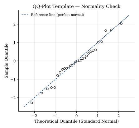
Normal Probability Plot (QQ-plot)
📖 해석만Unit 1Skill 4.B
X축
Theoretical (Normal) Quantiles 또는 z-score
Y축
Sample Quantiles 또는 변수값
판단
점들이 대각선 직선에 가까우면 정규분포 가정 적절
"approximately linear" → 정규성 만족
휘어짐(curve) → 비정규 (skew, heavy tails 등)
S자형 → tails 차이 / 두꺼움
⚠️ 출제 빈도: Stat에서는 정규성 검증 도구로 가끔 사용. boxplot/dotplot 모양과 함께 판단.
2
Mosaic Plot — 모자이크 그림
📖 해석만Unit 1·8Skill 4.B
축
두 범주형 변수 (각각 X·Y)
막대 폭
한 변수의 주변(marginal) 비율
막대 높이
다른 변수의 조건부(conditional) 비율
판단
모든 칸의 조건부 비율이 같으면 독립, 다르면 연관
CED 원문: "Bar graphs, side-by-side bar graphs, segmented bar graphs, and mosaic plots are examples of graphical representations." (CED p.65, Topic 1.6)
3
Time Series Plot — 시계열
📖 해석만Unit 1Skill 4.B
X축
Time (year, month, day 등)
Y축
측정변수 + 단위
점·선
시간순 연결
특징
trend (추세), seasonality (계절성), unusual features
4
Cumulative Frequency Plot — 누적빈도
📖 해석만Unit 1Skill 4.B
X축
변수값 (정렬)
Y축
Cumulative Frequency 또는 누적 백분율 (0~100%)
판단
Median = 50% 위치, Q1 = 25%, Q3 = 75% 위치를 X축으로 환산
곡선이 가파르면 데이터 밀집
완만하면 분산 큼
5
Side-by-side / Segmented Bar Graph — 그룹 비교 막대
📖 해석만Unit 1·8Skill 4.B
X축
범주 (각 그룹)
Y축
Frequency 또는 Relative Frequency / Proportion
막대
side-by-side: 그룹별 막대 분리 / segmented: 한 막대 안 색 분할 (합 = 1)
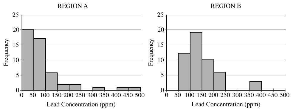
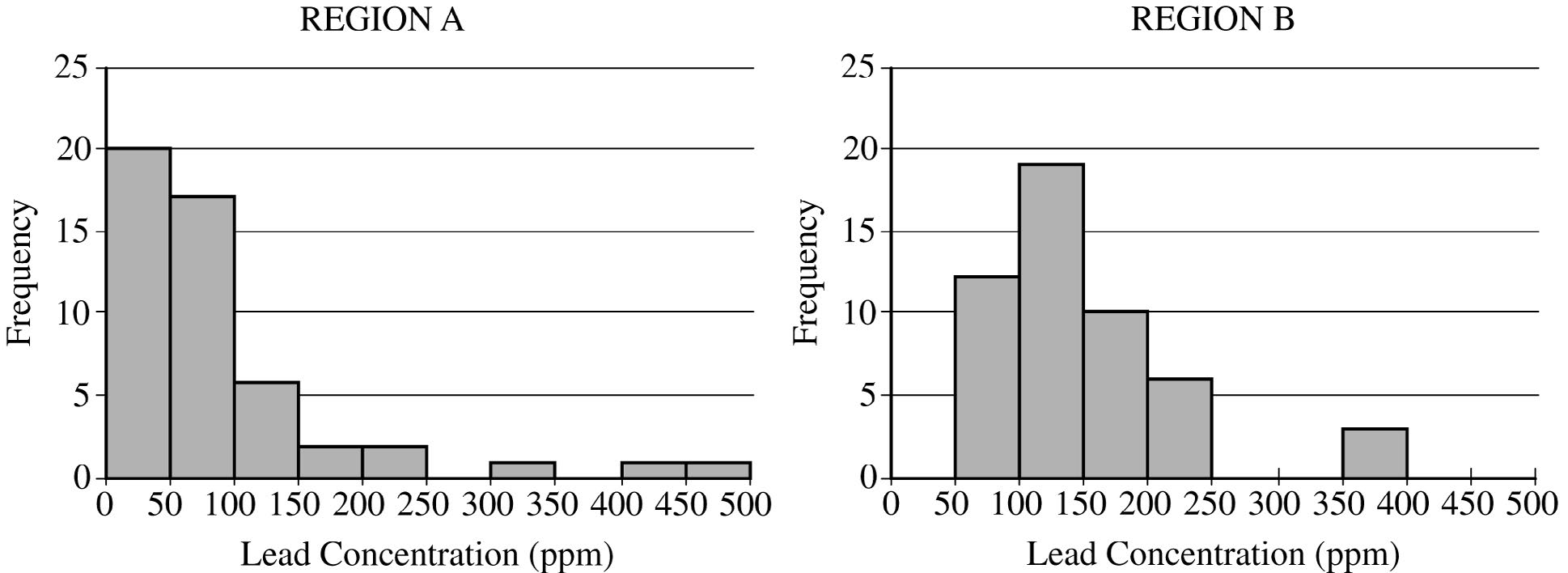
출처: AP Statistics CED · Sample FRQ Q1 · 인쇄 p.248 — 두 지역 lead concentration 분포 비교
📷 그래프 갤러리 — 28종 (출처별)
3개 출처에서 통합한 정연이용 그래프 라이브러리. 각 이미지는 data-source 속성으로 식별 가능. 직접 그리기 18개 카드 모두에 시각자료 매핑 완료 (3 → 18, 100%).
📌 중요: AP Statistics CED는 Econ과 달리 별도 "Graph Appendix"가 없다. 본 갤러리는 (1) CED PDF 자동 추출 9개(figure_extractor v2 + 원시 raster 추출), (2) 정연이 Mock Test 5 차용 7개, (3) 표준 수학 곡선 SVG 12개 합 28종. 출처 식별:data-source="ced"(College Board 원본 9) · data-source="borrowed"(차용 7, 출처: ap_stat_mock_test_5.html) · data-source="claude-svg"(Claude 합성 12, 검증 후 제거 가능).
📊 (A) CED PDF 추출 — 9개 (data-source="ced")
Sample Exam Questions(p.240·246·248·250 — 잔차도/히스토그램/분할표) + Formula Sheet 분포 곡선 4종.
1. Histograms (5 shapes) (Sample Q1, p.240)
2. Residual Plot (Sample Q15, p.246)
3. Side-by-side Histograms (FRQ Q1, p.247)
4. Residual Plot — Fan Pattern (Sample, p.245)
5. Lead Concentration Region A/B (HQ) (FRQ Q1, p.250 raw)
6. Standard Normal (Table A, p.262)
7. Standard Normal (continued) (Table A, p.263)
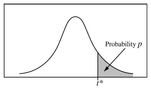
8. t-Distribution (Table B, p.265)
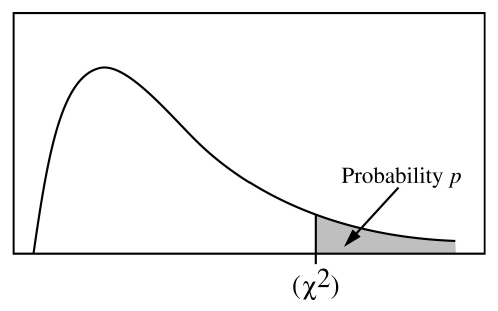
9. Chi-Square Distribution (Table C, p.267)
📂 (B) 정연이 Mock Test 5 차용 — 7개 (data-source="borrowed")
출처: ap_stat_mock_test_5.html — 본문 base64 이미지를 PNG로 분리해 같은 디렉토리에 보관 (CED 본문에 등장하지 않는 표준 그래프 형태 보강용).
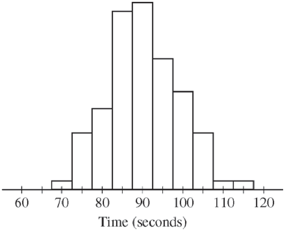
10. Histogram (Mice maze times) (Mock Q1)
11. Binomial PMF — 5 options (Mock Q14)
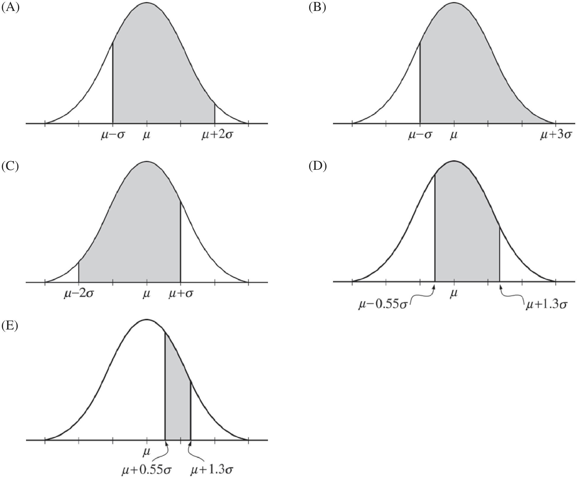
12. Normal — Shaded Regions (5 options) (Mock zucchini Q)
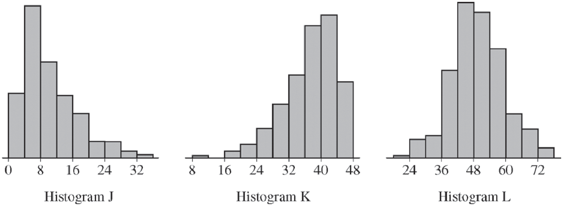
15. Histograms — Mean Position Comparison (Mock Q J/K/L)
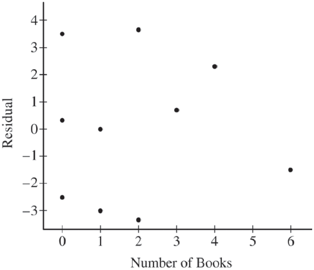
16. Residual Plot (Backpacks) (Mock Q regression)
🎨 (C) 표준 수학 곡선 SVG — 12개 (data-source="claude-svg")
CED·차용으로 채워지지 않는 이론 곡선만 합성 (특정 시나리오 데이터 X). matplotlib + scipy로 작성 후 ced_graphs/svg/에 보관. ※ Standard Normal·t-Dist·Binomial PMF는 PNG와 중복이라 명빈님 결정으로 제거(2026-05-02 13:36). 📌 명빈님께: 합성 SVG라 검증 후 제거 가능. 모든 이미지에 data-source="claude-svg" 속성으로 식별 가능.
17. Geometric PMF (p=0.3, μ=1/p)
18. QQ-Plot Template (정규성 가정)
19. CLT Visualization (n=2,10,30)
20. Sampling Dist. of p̂ (p=0.5, n=50)
21. Power Curve (α=0.05, n=30, target=0.80)
22. 95% CI Capture Demo (25 samples)
23. LSRL Template (scatterplot + 회귀선)
24. Cumulative Distribution (Ogive) (누적상대도수)
25. Sampling Dist. of x̄₁−x̄₂ (차이의 평균)
26. Dotplot Template (n=13, 수직 stacking) 🆕
27. Density — Symmetric vs Right-skewed (total area = 1) 🆕
28. Sampling Dist. of p̂₁−p̂₂ (차이의 비율, null=0) 🆕
📌 활용 팁: Stat에서는 축 라벨 정확성이 Econ보다 더 중요. ŷ vs y, p̂ vs p, x̄ vs μ — 모자/바 표기를 빼먹으면 통계 vs 모수 혼동으로 채점 시 의미 손실. CED 원본(A)을 우선으로 눈에 익히고, 차용(B)에서 추가 시각자료를 확인, SVG(C)는 표준 수학적 곡선 형태 학습용으로 활용.
⚠️ SVG (C) 검증 안내: Claude가 합성한 12개 SVG는 표준 형태(기하/QQ/CLT/Sampling Dist p̂·차이/Power/CI/LSRL/Cumulative/x̄₁−x̄₂/Dotplot/Density)만 포함. 데이터 시나리오는 들어가지 않음. 명빈님이 검증 후 제거하려면 ced_graphs/svg/ 디렉토리 삭제 + HTML에서 data-source="claude-svg" 항목만 제거하면 됨.
📋 종합 정리
18
직접 그리기 그래프
5
해석만 그래프
7
CED 원본 추출
🎯 시험 직전 1주 — 그래프 마스터 체크리스트
날짜
해야 할 것
D-5 (오늘)
이 페이지 1회 정독. 직접 그리기 18개의 X·Y축 라벨을 외운다. Histogram·Boxplot·Scatterplot·Residual Plot 4가지는 백지에 직접 그린다.
D-4
Sampling distribution 4종 (p̂, x̄, p̂₁−p̂₂, x̄₁−x̄₂) — 중심·SD 식 백지에 적기. Formula Sheet 보지 않고.
D-3
Normal / Binomial / Geometric / Density 곡선 모양·라벨. 음영(shaded area)으로 확률 표현하기.
D-2
Residual Plot 해석: "no apparent pattern" / "curved" / "fan-shaped" 표현 암기. CI / Power 시각화.
D-1
해석만 5개(QQ, Mosaic, Time series, Cumulative, Side-by-side bar) 빠르게 훑기. CED 원본 탭 정독.
D-0 (시험일)
이 페이지 30분 전 정독 + Formula Sheet 분포 곡선 그림 (p.262 / p.265 / p.267).